64 파이썬으로 회귀트리 구현하기
수치예측을 하는 의사결정트리를 사용하면 됨.
#1. 데이터 로드
#2. 결측치 확인
#3. 종속변수가 정규분포 보이는지 확인
#4. 훈련데이터 테스트데이터 분리
#5. 모델생성
#6. 모델훈련
#7. 모델예측
#8. 모델평가
#9. 모델성능개선
#python
#1. 데이터 로드
import pandas as pd
wine = pd.read_csv("c:\\data\\whitewines.csv")
wine.head()

#2. 결측치 확인
wine.isnull().sum()

#3. 종속변수가 정규분포 보이는지 확인
wine.quality.plot(kind = 'hist')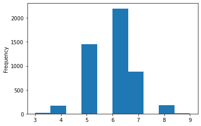
#4. 훈련데이터 테스트데이터 분리
from sklearn.model_selection import train_test_split

x = wine.iloc[:,:-1]
y = wine.iloc[:,-1]

x_train, x_test, y_train, y_test = train_test_split(x,y, test_size = 0.1, random_state = 1)

print(x_train.shape)  #(4408, 11)
print(x_test.shape)  #(490, 11)
print(y_train.shape)  #(4408,)
print(y_test.shape)  #(490,)

#5. 모델생성
from sklearn.tree import DecisionTreeRegressor

model = DecisionTreeRegressor(random_state = 1)

#6. 모델훈련
model.fit(x_train,y_train)

#7. 모델예측
result = model.predict(x_test)
result

#8. 모델평가
print(sum(result == y_test) / len(y_test)) # 정확도 0.610204081632653

#상관계수
import numpy as np
np.corrcoef(y_test, result)  # 0.58180875

#오차
def mae(x,y):
    return np.mean(abs(x-y))

print(mae(y_test, result))  #0.47551020408163264, R의 경우는 오차가 모델트리일때 0.57
from sklearn.ensemble import RandomForestClassifier 랜덤포레스트 분류
from sklearn.ensemble import RandomForestRegressor 랜덤포레스트 수치예측(회귀)
#9. 모델성능개선
from sklearn.ensemble import RandomForestRegressor  # 앙상블을 이용한 의사결정트리 회귀모델

model2 = RandomForestRegressor(random_state = 1)
model2.fit(x_train, y_train)  #모델훈련
result2 = model2.predict(x_test) #예측

sum(np.round(result2) == y_test) / len(y_test)  #정확도 0.6857142857142857

np.corrcoef(result2, y_test)  #상관계수 0.71178998

mae(y_test, result2) #오차 0.4348979591836732
ㅇ파이썬에서 수치예측하는 모델 패키지 정리
1. 다중회귀모델
: from sklearn.linear_model import LinearRegression
2. 의사결정트리 회귀모델
: from sklearn.tree import DecisionTreeRegressor
3. 랜덤포레스트 회귀모델
: from sklearn.ensemble import RandomForestRegressor
문제323. 미국 보스톤 지역의 집값을 예측하는 회귀모델을 만드는데 다중회귀 모델인 LinearRegression으로 모델을 만들고 성능을 확인하시오.
#1. 데이터 로드
import pandas as pd

boston = pd.read_csv("c:\\data\\boston.csv")
boston.head()

#2. 결측치 확인
boston.isnull().sum()

#3. 종속변수가 정규분포 보이는지 확인
boston.price.plot(kind = 'hist')
#4. 훈련데이터 테스트데이터 분리
from sklearn.model_selection import train_test_split

x = boston.iloc[:,:-1]
y = boston.iloc[:,-1]

x_train, x_test, y_train, y_test = train_test_split(x,y, test_size = 0.1, random_state = 1)

print(x_train.shape, x_test.shape, y_train.shape, y_test.shape)  #(455, 14) (51, 14) (455,) (51,)

#다중회귀모델
#5. 모델생성
from sklearn.linear_model import LinearRegression

model = LinearRegression()

#6. 모델훈련
model.fit(x_train, y_train)

#7. 모델예측
result = model.predict(x_test)

#8. 모델평가
import numpy as np
print(np.corrcoef(y_test, result))  #상관계수 0.88804528
print(mae(y_test, result))  #오차 3.7468103368637924
이번에는 의사결정트리 회귀모델(from sklearn.tree import DecisionTreeRegressor)로 진행해보자.
# 의사결정트리 회귀모델
#5. 모델생성
from sklearn.tree import DecisionTreeRegressor

model2 = DecisionTreeRegressor(random_state = 1)

#6. 모델훈련
model2.fit(x_train, y_train)

#7. 모델예측
result2 = model2.predict(x_test)

#8. 모델평가
print(np.corrcoef(y_test,result2))  #상관계수 0.93594231
print(mae(y_test,result2))  #오차 2.509803921568628
문제325. 그럼 이번에는 RandomForestRegressor로 구현해서 성능을 평가하시오.
#랜덤포레스트 회귀모델
#5. 모델생성
from sklearn.ensemble import RandomForestRegressor

model3 = RandomForestRegressor(random_state = 1)

#6. 모델훈련
model3.fit(x_train, y_train)

#7. 모델예측
result3 = model3.predict(x_test)

#8. 모델평가
print(np.corrcoef(y_test,result3))  #상관계수 0.96688151
print(mae(y_test,result3))  #오차 1.927784313725491
| 상관계수 | 오차 | |
| 다중회귀모델 | 0.88804528 | 3.7468103368637924 |
| 의사결정트리 회귀모델 | 0.93594231 | 2.509803921568628 |
| 랜덤포레스트 회귀모델 | 0.96688151 | 1.927784313725491 |
> 랜덤포레스트 회귀모델의 성능이 가장 좋음.
반응형
'Study > class note' 카테고리의 다른 글
| [스터디] 로지스틱스회귀 스터디 (0) | 2022.02.16 |
|---|---|
| 머신러닝 / 신경망 이론 (0) | 2022.02.16 |
| 머신러닝 / R 로 회귀트리 구현하기, R 로 모델트리 구현하기 (0) | 2022.02.16 |
| 머신러닝 / 회귀트리 (0) | 2022.02.15 |
| 머신러닝 / 다중공선성 실험하기(R 과 파이썬), 다중회귀분석 모델을 파이썬을 구현 (0) | 2022.02.15 |

