ㅇ복습
1장. numpy와 matplotlib
2장. 퍼셉트론
3장. 저자가 만들어온 가중치로 3층 신경망을 생성
4장. 우리가 직접 학습이 가능한 2층 신경망을 생성(수치미분)
5장. 우리가 직접 학습이 가능한 2층 신경망을 생성(오차역전파)
14 파이썬 날코딩으로 2층 신경망 전체 코드 구현 - p180
문제120. 어제 만들었던 2층 신경망 설계도(클래스)를 가지고 net이라는 객체를 만드시오.
import sys, os
sys.path.append(os.pardir)  # 부모 디렉터리의 파일을 가져올 수 있도록 설정
from common.functions import *
from common.gradient import numerical_gradient

class TwoLayerNet:
    def __init__(self, input_size, hidden_size, output_size, weight_init_std=0.01):
        # 가중치 초기화
        self.params = {}
        self.params['W1'] = weight_init_std * np.random.randn(input_size, hidden_size)
        self.params['b1'] = np.zeros(hidden_size)
        self.params['W2'] = weight_init_std * np.random.randn(hidden_size, output_size)
        self.params['b2'] = np.zeros(output_size)

    def predict(self, x):
        W1, W2 = self.params['W1'], self.params['W2']
        b1, b2 = self.params['b1'], self.params['b2']
        a1 = np.dot(x, W1) + b1
        z1 = sigmoid(a1)
        a2 = np.dot(z1, W2) + b2
        y = softmax(a2)
        return y

    # x : 입력 데이터, t : 정답 레이블
    def loss(self, x, t):
        y = self.predict(x)
        return cross_entropy_error(y, t)

    def accuracy(self, x, t):
        y = self.predict(x)
        y = np.argmax(y, axis=1)
        t = np.argmax(t, axis=1)

        accuracy = np.sum(y == t) / float(x.shape[0])
        return accuracy


    # x : 입력 데이터, t : 정답 레이블
    def numerical_gradient(self, x, t):
        loss_W = lambda W: self.loss(x, t)

        grads = {}
        grads['W1'] = numerical_gradient(loss_W, self.params['W1'])
        grads['b1'] = numerical_gradient(loss_W, self.params['b1'])
        grads['W2'] = numerical_gradient(loss_W, self.params['W2'])
        grads['b2'] = numerical_gradient(loss_W, self.params['b2'])

        return grads

    def gradient(self, x, t):
        W1, W2 = self.params['W1'], self.params['W2']
        b1, b2 = self.params['b1'], self.params['b2']
        grads = {}

        batch_num = x.shape[0]

        # forward
        a1 = np.dot(x, W1) + b1
        z1 = sigmoid(a1)
        a2 = np.dot(z1, W2) + b2
        y = softmax(a2)

        # backward
        dy = (y - t) / batch_num
        grads['W2'] = np.dot(z1.T, dy)
        grads['b2'] = np.sum(dy, axis=0)

        da1 = np.dot(dy, W2.T)
        dz1 = sigmoid_grad(a1) * da1
        grads['W1'] = np.dot(x.T, dz1)
        grads['b1'] = np.sum(dz1, axis=0)
        return grads
net = TwoLayerNet(input_size = 768, hidden_size = 100, output_size = 10)
net
문제121. 위의 2층 신경망에 입력할 학습 데이터로 텐서플로우 2.0에 내장된 mnist 데이터를 입력데이터로 구성하시오.
#2. 필기체 데이터 로드
from tensorflow.keras.datasets.mnist import load_data

(x_train, y_train), (x_test, y_test) = load_data(path='mnist.npz')

print(x_train.shape)  #(60000, 28, 28)
문제122. 텐서플로우에서 불러온 3차원 mnist데이터를 2차원으로 변경하시오.
#3. 입력데이터 구성(3차원 -> 2차원)
x_train = x_train.reshape(60000,28*28)
x_train = x_train / 255 #정규화

print(x_train.shape)  #(60000, 784)
문제123. 정답 데이터를 구성하시오.(원핫인코딩)
#4. 정답데이터를 구성
from  tensorflow.keras.utils  import  to_categorical

y_train = to_categorical(y_train)  #원핫인코딩

print(y_train.shape)  #(60000, 10)
문제124. 필기체 데이터 300장만 신경망에 넣고 학습시키시오.
#5. 신경망 학습
for i in range(3):
    batch_mask = np.random.choice(60000,100)  #0부터 60000까지의 숫자 중에서 100개의 숫자를 랜덤으로 추출
    x_batch = x_train[batch_mask]  #100개의 이미지 데이터 추출
    t_batch = y_train[batch_mask]  #100개의 정답 데이터를 추출
    grad = net.gradient(x_batch, t_batch)  # 기울기 추출
    print(grad)
문제125. 학습이 되고 있는지 확인하기 위해서 오차를 출력하시오.
#5. 신경망 학습
train_loss_list = []

for i in range(3):
    batch_mask = np.random.choice(60000,100)  #0부터 60000까지의 숫자 중에서 100개의 숫자를 랜덤으로 추출
    x_batch = x_train[batch_mask]  #100개의 이미지 데이터 추출
    t_batch = y_train[batch_mask]  #100개의 정답 데이터를 추출
    grad = net.gradient(x_batch, t_batch)  # 기울기 추출

    for key in ('W1','b1','W2','b2'):
        net.params[key] -= 0.1*grad[key]  #학습률 0.1 * 기울기를 빼줌
    loss = net.loss(x_batch, t_batch) #오차함수에 100장의 이미지와 100장의 정답을 넣어서 오차를 loss에 넣습니다.
    train_loss_list.append(loss) # 오차를 train_loss_list에 append 시킵니다.

print(train_loss_list)  #[2.2910370336825023, 2.2866595156070177, 2.2853408481217232]
문제126. 위에서는 300장만 학습 시켰는데 6만장을 전부 학습 시키시오.
#5. 신경망 학습
train_loss_list = []

for i in range(600):
    batch_mask = np.random.choice(60000,100)  #0부터 60000까지의 숫자 중에서 100개의 숫자를 랜덤으로 추출
    x_batch = x_train[batch_mask]  #100개의 이미지 데이터 추출
    t_batch = y_train[batch_mask]  #100개의 정답 데이터를 추출
    grad = net.gradient(x_batch, t_batch)  # 기울기 추출

    for key in ('W1','b1','W2','b2'):
        net.params[key] -= 0.1*grad[key]  #학습률 0.1 * 기울기를 빼줌
    loss = net.loss(x_batch, t_batch) #오차함수에 100장의 이미지와 100장의 정답을 넣어서 오차를 loss에 넣습니다.
    train_loss_list.append(loss) # 오차를 train_loss_list에 append 시킵니다.
문제127. 1에폭당 오차 하나가 출력되게 코드를 수정하시오.
#5. 신경망 학습
train_loss_list = []

for i in range(600):
    batch_mask = np.random.choice(60000,100)  #0부터 60000까지의 숫자 중에서 100개의 숫자를 랜덤으로 추출
    x_batch = x_train[batch_mask]  #100개의 이미지 데이터 추출
    t_batch = y_train[batch_mask]  #100개의 정답 데이터를 추출
    grad = net.gradient(x_batch, t_batch)  # 기울기 추출

    for key in ('W1','b1','W2','b2'):
        net.params[key] -= 0.1*grad[key]  #학습률 0.1 * 기울기를 빼줌

    if (i+1) % 600 == 0:
        loss = net.loss(x_batch, t_batch) #오차를 loss에 넣습니다.
        train_loss_list.append(loss) # 오차를 train_loss_list에 append 시킵니다.

print(train_loss_list)
문제128. 이제 위의 코드를 30에폭 돌리게끔 코드를 수정하시오.
#5. 신경망 학습
train_loss_list = []

epochs = 600* 30  # 30에폭

for i in range(epochs):
    batch_mask = np.random.choice(60000,100)  #0부터 60000까지의 숫자 중에서 100개의 숫자를 랜덤으로 추출
    x_batch = x_train[batch_mask]  #100개의 이미지 데이터 추출
    t_batch = y_train[batch_mask]  #100개의 정답 데이터를 추출
    grad = net.gradient(x_batch, t_batch)  # 기울기 추출

    for key in ('W1','b1','W2','b2'):
        net.params[key] -= 0.1*grad[key]  #학습률 0.1 * 기울기를 빼줌

    if (i+1) % 600 == 0:
        loss = net.loss(x_batch, t_batch) #오차를 loss에 넣습니다.
        train_loss_list.append(loss) # 오차를 train_loss_list에 append 시킵니다.

print(train_loss_list)
문제129. 이번에는 정확도를 비어있는 리스트 train_acc_list에 append 시키시오.
#6. 정확도
train_loss_list = []
train_acc_list = []

epochs = 600* 30  # 30에폭

for i in range(epochs):
    batch_mask = np.random.choice(60000,100)  #0부터 60000까지의 숫자 중에서 100개의 숫자를 랜덤으로 추출
    x_batch = x_train[batch_mask]  #100개의 이미지 데이터 추출
    t_batch = y_train[batch_mask]  #100개의 정답 데이터를 추출
    grad = net.gradient(x_batch, t_batch)  # 기울기 추출

    for key in ('W1','b1','W2','b2'):
        net.params[key] -= 0.1*grad[key]  #학습률 0.1 * 기울기를 빼줌

    if (i+1) % 600 == 0:
        loss = net.loss(x_batch, t_batch) #오차를 loss에 넣습니다.
        train_loss_list.append(loss) # 오차를 train_loss_list에 append 시킵니다.
        train_acc = net.accuracy(x_train, y_train)  #훈련데이터와 훈련데이터의 정답을 넣고 훈련데이터의 정확도를 담음.
        train_acc_list.append(train_acc)

print(train_loss_list)
print(train_acc_list)
문제130. 지금 train_acc_list에 담긴 정확도를 시각화 하시오.
import matplotlib.pyplot as plt

x = np.arange(len(train_acc_list))
plt.plot(x, train_acc_list, label = 'train_acc')
plt.ylim(0.9,1)
plt.show()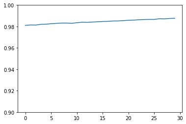
문제131. 이번에는 훈련데이터의 정확도를 구하는 것과 동시에 테스트 데이터에 대한 정확도도 test_acc_list에 담기게 하시오.
#3. 입력데이터 정규화
x_test = x_test.reshape(10000, 28*28)
x_test = x_test/255

#4. 정답 데이터 구성
y_test =to_categorical(y_test)

#6. 정확도
train_loss_list = []
train_acc_list = []
test_acc_list = []

epochs = 600* 30  # 30에폭

for i in range(epochs):
    batch_mask = np.random.choice(60000,100)  #0부터 60000까지의 숫자 중에서 100개의 숫자를 랜덤으로 추출
    x_batch = x_train[batch_mask]  #100개의 이미지 데이터 추출
    t_batch = y_train[batch_mask]  #100개의 정답 데이터를 추출
    grad = net.gradient(x_batch, t_batch)  # 기울기 추출

    for key in ('W1','b1','W2','b2'):
        net.params[key] -= 0.1*grad[key]  #학습률 0.1 * 기울기를 빼줌

    if (i+1) % 600 == 0:
        loss = net.loss(x_batch, t_batch) #오차를 loss에 넣습니다.
        train_loss_list.append(loss) # 오차를 train_loss_list에 append 시킵니다.
        train_acc = net.accuracy(x_train, y_train)  #훈련데이터와 훈련데이터의 정답을 넣고 훈련데이터의 정확도를 담음.
        test_acc = net.accuracy(x_test, y_test)  #훈련데이터와 훈련데이터의 정답을 넣고 훈련데이터의 정확도를 담음.
        train_acc_list.append(train_acc)
        test_acc_list.append(test_acc)

print(train_loss_list)
print(train_acc_list)
print(test_acc_list)
문제132. train_acc_list와 test_acc_list에 담긴 두 개의 정확도를 아래와 같이 시각화 하시오.
import matplotlib.pyplot as plt
x = np.arange(len(train_acc_list))
plt.plot(x, train_acc_list, label='train_acc')
plt.plot(x, test_acc_list, label='test_acc', linestyle = '--')

plt.ylim(0.8,1)
plt.xlabel('epochs')
plt.ylabel('accuracy')
plt.legend()
plt.show()
+) 지금까지 한 코드 전체정리
# 클래스 생성
import sys, os
sys.path.append(os.pardir)  # 부모 디렉터리의 파일을 가져올 수 있도록 설정
from common.functions import *
from common.gradient import numerical_gradient

class TwoLayerNet:
    def __init__(self, input_size, hidden_size, output_size, weight_init_std=0.01):
        # 가중치 초기화
        self.params = {}
        self.params['W1'] = weight_init_std * np.random.randn(input_size, hidden_size)
        self.params['b1'] = np.zeros(hidden_size)
        self.params['W2'] = weight_init_std * np.random.randn(hidden_size, output_size)
        self.params['b2'] = np.zeros(output_size)

    def predict(self, x):
        W1, W2 = self.params['W1'], self.params['W2']
        b1, b2 = self.params['b1'], self.params['b2']
        a1 = np.dot(x, W1) + b1
        z1 = sigmoid(a1)
        a2 = np.dot(z1, W2) + b2
        y = softmax(a2)
        return y

    # x : 입력 데이터, t : 정답 레이블
    def loss(self, x, t):
        y = self.predict(x)
        return cross_entropy_error(y, t)

    def accuracy(self, x, t):
        y = self.predict(x)
        y = np.argmax(y, axis=1)
        t = np.argmax(t, axis=1)

        accuracy = np.sum(y == t) / float(x.shape[0])
        return accuracy


    # x : 입력 데이터, t : 정답 레이블
    def numerical_gradient(self, x, t):
        loss_W = lambda W: self.loss(x, t)

        grads = {}
        grads['W1'] = numerical_gradient(loss_W, self.params['W1'])
        grads['b1'] = numerical_gradient(loss_W, self.params['b1'])
        grads['W2'] = numerical_gradient(loss_W, self.params['W2'])
        grads['b2'] = numerical_gradient(loss_W, self.params['b2'])

        return grads

    def gradient(self, x, t):
        W1, W2 = self.params['W1'], self.params['W2']
        b1, b2 = self.params['b1'], self.params['b2']
        grads = {}

        batch_num = x.shape[0]

        # forward
        a1 = np.dot(x, W1) + b1
        z1 = sigmoid(a1)
        a2 = np.dot(z1, W2) + b2
        y = softmax(a2)

        # backward
        dy = (y - t) / batch_num
        grads['W2'] = np.dot(z1.T, dy)
        grads['b2'] = np.sum(dy, axis=0)

        da1 = np.dot(dy, W2.T)
        dz1 = sigmoid_grad(a1) * da1
        grads['W1'] = np.dot(x.T, dz1)
        grads['b1'] = np.sum(dz1, axis=0)
        return grads


#1. 객체 생성
net = TwoLayerNet(input_size = 784, hidden_size = 100, output_size = 10)

#2. 필기체 데이터 로드
from tensorflow.keras.datasets.mnist import load_data

(x_train, y_train), (x_test, y_test) = load_data(path='mnist.npz')

#3. 입력데이터 구성(3차원 -> 2차원)
x_train = x_train.reshape(60000,28*28)
x_train = x_train / 255 #정규화

x_test = x_test.reshape(10000,28*28)
x_test = x_test / 255

#4. 정답데이터를 구성
from  tensorflow.keras.utils  import  to_categorical

y_train = to_categorical(y_train)  #원핫인코딩
y_test = to_categorical(y_tet)

#5. 훈련 및 평가
train_loss_list = []
train_acc_list = []
test_acc_list = []

epochs = 600* 30  # 30에폭

for i in range(epochs):
    batch_mask = np.random.choice(60000,100)  #0부터 60000까지의 숫자 중에서 100개의 숫자를 랜덤으로 추출
    x_batch = x_train[batch_mask]  #100개의 이미지 데이터 추출
    t_batch = y_train[batch_mask]  #100개의 정답 데이터를 추출
    grad = net.gradient(x_batch, t_batch)  # 기울기 추출

    for key in ('W1','b1','W2','b2'):
        net.params[key] -= 0.1*grad[key]  #학습률 0.1 * 기울기를 빼줌

    if (i+1) % 600 == 0:
        loss = net.loss(x_batch, t_batch) #오차를 loss에 넣습니다.
        train_loss_list.append(loss) # 오차를 train_loss_list에 append 시킵니다.
        train_acc = net.accuracy(x_train, y_train)  #훈련데이터와 훈련데이터의 정답을 넣고 훈련데이터의 정확도를 담음.
        test_acc = net.accuracy(x_test, y_test)  #훈련데이터와 훈련데이터의 정답을 넣고 훈련데이터의 정확도를 담음.
        train_acc_list.append(train_acc)
        test_acc_list.append(test_acc)

print(train_loss_list)
print(train_acc_list)
print(test_acc_list)
'Study > class note' 카테고리의 다른 글
| 딥러닝 / 언더피팅 방지(가중치 초기값, 배치정규화) (0) | 2022.04.13 |
|---|---|
| 딥러닝 / 2층 신경망을 텐서 플로우로 구현 (0) | 2022.04.13 |
| 딥러닝 / 오차역전파, Affine 계층 구현 (0) | 2022.04.12 |
| 딥러닝 / 오차역전파를 이용한 2층 신경망 구현 (0) | 2022.04.11 |
| 딥러닝 / 패션 mnist 신경망에 사진을 넣고 잘 예측하는지 확인하기(+구글 코랩) (0) | 2022.04.10 |


